Section 1.1
- 在图像中直线保持原来的特征,而诸如形状、角度、距离、比例则会发生改变
Part 0 Outline
- Chapter 2 introduces projective transformations of 2-space.
- Chapter 3 covers the projective geometry of 3-space.
- Chapter 4 introducesestimationof geometry from image m easureme
- Chapter 5 describes how the results of estimation algorithms may be evaluated
Section 2.1 - 2.2.2
Homogeneous representation
lines
points

Result2.1

Note:

Degrees of freedom / DOF
Intersection of lines

Line joining points

Intersection of parallel lines
- \((0,1,0)^T\)即在y轴方向的infinity
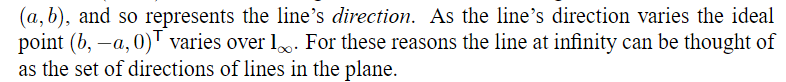
Ideal points and the line at infinity
In inhomogeneous notation \((b,-a)^T\) is a vector tangent to the line \((a,b,c)^t\), and orthogonal to the line normal \((a,b)\), and so represents the line's direction.
- points at infinity ==> in the projective plane \(\mathbb{P}^2\), one may state without qualification two distinct lines meet in a single point and tow distinct points lie on a line.
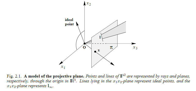
A model of the projective plane
Duality / Duality Principle (p30)
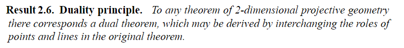
- concepts of incidence must be appropriately translated aswell. For instance, the line through two points is dual to the point through (that is thepoint of intersection of) two lines.
Section 2.2.3
Conics and dual Conics
In Euclideangeometry conics are of three main types: hyperbola, ellipse, and parabola (apart fromso-called degenerate conics, to be defined later).
- The equation of a conic in inhomogeneous coordinates is $ ax2+bxy+cy2+dx+ey+f=0 $(i.e. a polynomial of degree 2.)
"Homogenizing" the equation above by the replacements:\(x \mapsto x_1/x_3, y \mapsto x_2/x_3\) gives
\(a x_1^2 + b x_1 x_2 + c x_2^2 + d x_1 x_3 + e x_2 x_3 + f x_3^2 = 0\)
or in matrix form: \(\mathbf{x}^T C \mathbf{x} = 0\)
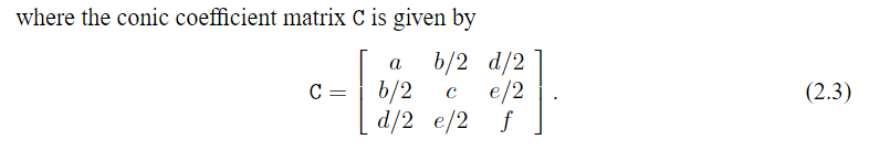
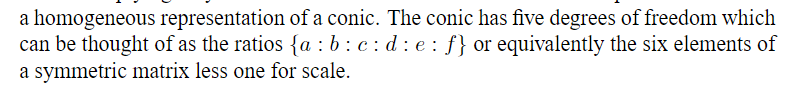
C in \((2.3)\) is a homogeneous representation of a conic.
Since multiplyingCby a non-zero scalar does not affect the above equations, only the ratios of the matrix elements are important.
DOF : 5
DOF ==> Five points define a conic
Tangle lines to Conics

Dual conics
The conic \(C\) defined above is more properly termed a point conic, as it defines an equation on points.
an equation on points ==> an equation on lines
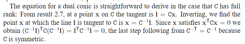
This dual / line conic is represented by \(3 \times 3\) matrix \(C^*\)
A line \(l\) tangle to the conic C statisfies \(l^T C^* l =0\)
For a non-singular symmetric matrix \(C^∗=C^{−1}\)(up to scale).
prove:
DOF: 5
Degenerate conics
If the matrix \(C\) is not of full rank, then the conic is termed degenerate. Degenerate point conics include two lines (rank 2), and a repeated line (rank 1).
Section 2.3 Projective transformations
Geometry is the study of properties invariant under groups of transformations.
- ==> 2D Projective geometry is the study of properties of the projective plane \(\mathbb{P}^2\) that are invariant under a group of transformations known as projectivities.
Definition of projectivity
Definition 2.9

Projectivities form a group since the inverse of a projectivity is also a projectivity, and so is the composition of two projectivities.
A projectivity is also called a collineation(a helpful name), a projective transformation or a homography.
An equivalent algebraic Definition
- Any invertible linear transformation of homogeneous coordinates is a projectivity.
Theorem 2.10.
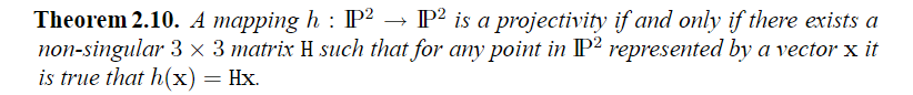
==> Another alternative definition of a projective transformation
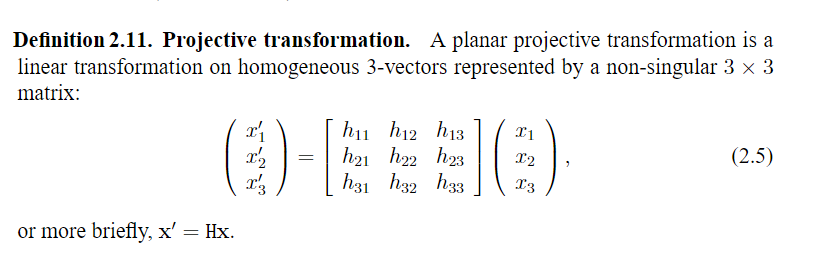
\(H\) is a homogeneous matrix, since as in the homogeneous representation of a point, only the ratio of the matrix elements is significant.
DOF of \(H\) : 8
Mappings between planes
Central projection maps points on one plane to points on another plane.
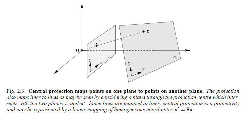
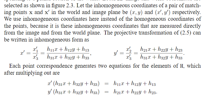
If a coordinate system is defined in each plane and points are represented in homogeneous coordinates, then the central projection mapping may be expressed by \(x'=H x\).
If the two coordinate systems defined in the two planes are both Euclidean(rectilinear) coordinate systems then the mapping defined by projection is more restricted than an arbitrart projective transformation. It is called a prespectivity rather than a full projectivity, and may be represented by a transformation with six degrees of freedom.
Example 2.12 :Removing the projective distortion from a perspective image of a plane.
Three remarks concerning this example are appropriate
- The computation of the rectifying transformation \(H\) in this way does not require knowledge of any of the camera’s parameters or the pose of the plane
- It is not always necessary to know coordinates for four points in order to remove projective distortion: alternative approaches, which are described in section 2.7, require less, and different types of, information
- Superior (and preferred) methods for computing projective transfor-mations are described in chapter 4.
2.3.1 Transformations of lines and conics
Transformation of lines
Under the point transformation \(x' = Hx\), a line transforms as
\[ \mathbb{l}'=H^{-T} \mathbb{l} \]
Points transform according to \(H\), where as lines(as rows) transform according to \(H^{−1}\).
- This may be explained in terms of "covariant" or "contravariant" behaviour. One says that points transform contravariantly and lines transform covariantly.
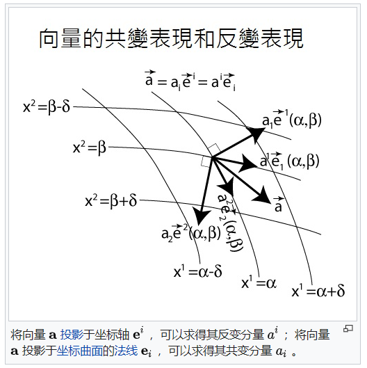
- This may be explained in terms of "covariant" or "contravariant" behaviour. One says that points transform contravariantly and lines transform covariantly.
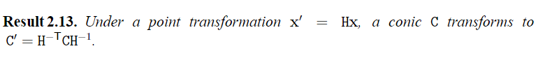
Transformation of conics
Under a point transformation \(x′=Hx\),